Logistic Regression With a Single Continuous Predictor Variable Python

In Machine Learning, we often need to solve problems that require one of the two possible answers, for example in the medical domain, we might be looking to find whether a tumor is malignant or benign and similarly in the education domain, we might want to see whether a student gets admission in a specific university or not.

Such problems are binary classification problems and logistic regression is a very popular algorithm to solve such problems. With that said, it would be easier to understand what logistic regression is.

What is Logistic Regression?

Logistic Regression is a Machine Learning algorithm used to make predictions to find the value of a dependent variable such as the condition of a tumor (malignant or benign), classification of email (spam or not spam), or admission into a university (admitted or not admitted) by learning from independent variables (various features relevant to the problem).

For example, for classifying an email, the algorithm will use the words in the email as features and based on that make a prediction whether the email is spam or not.

Logistic Regression is a supervised Machine Learning algorithm, which means the data provided for training is labeled i.e., answers are already provided in the training set. The algorithm learns from those examples and their corresponding answers (labels) and then uses that to classify new examples.

In mathematical terms, suppose the dependent variable is Y and the set of independent variables is X, then logistic regression will predict the dependent variable P(Y=1) as a function of X, the set of independent variables.

Types of Logistic Regression

When we talk about Logistic Regression in general, we usually mean Binary logistic regression, although there are other types of Logistic Regression as well.

Logistic Regression can be divided into types based on the type of classification it does. With that in view, there are 3 types of Logistic Regression. Let's talk about each of them:

• Binary Logistic Regression
• Multinomial Logistic Regression
• Ordinal Logistic Regression

Binary Logistic Regression

Binary Logistic Regression is the most commonly used type. It is the type we already discussed when defining Logistic Regression. In this type, the dependent/target variable has two distinct values, either 0 or 1, malignant or benign, passed or failed, admitted or not admitted.

Multinomial Logistic Regression

Multinomial Logistic Regression deals with cases when the target or independent variable has three or more possible values. For example, the use of Chest X-ray images as features that give indication about one of the three possible outcomes (No disease, Viral Pneumonia, COVID-19). The multinomial Logistic Regression will use the features to classify the example into one of the three possible outcomes in this case. There can of course be more than three possible values of the target variable.

Ordinal Logistic Regression

Ordinal Logistic Regression is used in cases when the target variable is of ordinal nature. In this type, the categories are ordered in a meaningful manner and each category has quantitative significance. Moreover, the target variable has more than two categories. For example, the grades obtained on an exam have categories that have quantitative significance and they are ordered. Keeping it simple, the grades can be A, B, or C.

Difference between Logistic and Linear Regression

The major difference between Logistic and Linear Regression is that Linear Regression is used to solve regression problems whereas Logistic Regression is used for classification problems. In regression problems, the target variable can have continuous values such as the price of a product, the age of a participant, etc. While, the classification problems deal with the prediction of target variable that can only have discrete values, for example, prediction of gender of a person, prediction of a tumor to be malignant or benign, etc.

In what type of software does logistic regression work best?

Logistic Regression is most commonly used in problems of binary classification in which the algorithm predicts one of the two possible outcomes based on various features relevant to the problem.

Logistic Regression finds its applications in a wide range of domains and fields, the following examples will highlight its importance:

Education sector: In the Education sector, logistic regression can be used to predict:

• Whether a student gets admission into a university program or not is based on test scores and various other factors.
• In E-learning platforms to see whether a student will complete a course on time or not based on past activity and other statistics relevant to the problem.

Business sector: In the business sector, logistic regression has the following applications:

• Predicting whether a credit card transaction made by a user is fraudulent or not.

Medical sector: Medical sector also benefits from logistic regression through the following uses:

• Predicting whether a person has a disease or not is based on values obtained from test reports or other factors in general.
• A very innovative application of Machine Learning being used by researchers is to predict whether a person has COVID-19 or not using Chest X-ray images.

Other applications: Logistic regression finds its applications in all major sectors, in addition to that, some of its interesting applications are:

• Email Classification – Spam or not spam
• Sentiment Analysis – Person is sad or happy based on a text message
• Object Detection and Classification – Classifying an image to be a cat image or a dog image

There are numerous other problems that can be solved using Logistic Regression. The above-mentioned examples should be enough to give you an idea of how powerful and useful this algorithm is.

Example of Algorithm based on Logistic Regression and its implementation in Python

Now that the basic concepts about Logistic Regression are clear, it is time to study a real-life application of Logistic Regression and implement it in Python.

Let's work on classifying credit card transactions as fraudulent, also called credit card fraud detection. It is a very important application of Logistic Regression being used in the business sector. A real-world dataset will be used for this problem. It is quite a comprehensive dataset having information of over 280,000 transactions. Step by step instructions will be provided for implementing the solution using logistic regression in Python.

So let's get started:

Step 1 – Doing Imports

The first step is to import the libraries that are going to be used later. If you do not have them installed, you would have to install them using pip or any other package manager for python.

          import pandas as pd  from sklearn.model_selection import train_test_split  from sklearn.linear_model import LogisticRegression  from sklearn import preprocessing  from sklearn.metrics import accuracy_score, classification_report, confusion_matrix  from matplotlib import pyplot as plt  import seaborn as sns        

Step 2 – The Data

The second step is to get data that is going to be used for the analysis and then perform preprocessing steps on the data.

Step 2.1 – Downloading the Data

The dataset to be used in this example can be downloaded from Kaggle. After downloading, the archive would have to be extracted and the CSV file would be obtained.

Step 2.2 – Loading the data using Pandas

The CSV file is placed in the same directory as the jupyter notebook (or code file), and then the following code can be used to load the dataset:

          df = pd.read_csv('creditcard.csv')        

Pandas will load the CSV file and form a data structure called a Pandas Data Frame. It is conventional to name the Data Frame as 'df', but it can be named anything meaningful and relevant to the data as well.

Step 2.3 – Exploring the Data

After loading the data, the dataset can be explored to understand it better.

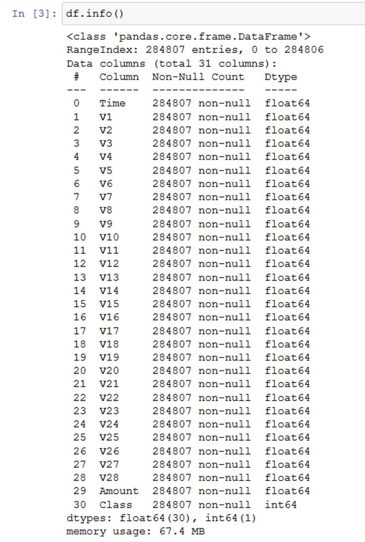
The dataset contains 30 columns, Class is the target variable, while all others are features of the dataset. The most important variables are named from V1 to V28.

Looking at the first few rows of the dataset.

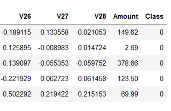
Not all columns can be displayed at once on the screen, therefore the remaining ones are shown below:

Step 2.4 – Preprocessing the Dataset

Preprocessing the dataset is a very important part of the analysis, it is used to remove outliers and duplicates from the dataset. Moreover, it is a very common practice to scale the columns on a standard scale, it helps in faster convergence and gives better results.

Looking at the number of duplicate rows in the dataset:

There are over a thousand duplicate rows that should be removed from the dataset. Therefore, removing the duplicates using the line of code below:

          df.drop_duplicates(inplace=True)        

In addition to rows, sometimes there are columns in the data which do not give any meaningful information for the classification, therefore they should be removed from the data before training the model. One such column in our dataset is the Time column. It can be removed using the line of code given below:

          df.drop('Time', axis=1, inplace=True)        

After the data has been cleaned, the dataset columns can be separated into feature columns and target column. As mentioned before, the class column is the target column and everything else is a feature. Thus, doing that below:

          X = df.iloc[:,df.columns != 'Class'] y = df.Class                  

Having done that, the dataset can be divided into training and test sets. The training set is used to train the classifier, while the test set can be used to evaluate the performance of the classifier on unseen instances.

          X_train, X_test, y_train, y_test = train_test_split( X, y, test_size=0.20, random_state=5, stratify=y)        

Before supplying the data to the classifier, the dataset is scaled using a standard scalar (as mentioned before). It is done using the code below:

          scaler = preprocessing.StandardScaler().fit(X_train) X_train_scaled = scaler.transform(X_train)                  

This completes our preprocessing of the dataset. Note that preprocessing often determines the success or failure of analysis and therefore should be taken very seriously. Various other things are done during the preprocessing stage depending on the type and nature of data, but this brief overview should be enough to give an idea about how it works.

Step 3 – Exploratory Data Visualization

It often makes things much easier to understand when visualizations and graphics are used. The same goes for Machine Learning problems. Different aspects of the dataset are visualized to get a better understanding of the data, and this process is called exploratory data visualization.

Plotting histograms to understand the values of each variable is a good place to start. Using the code given below:

          import matplotlib.colors as mcolors colors = list(mcolors.CSS4_COLORS.keys())[10:] def draw_histograms(dataframe, features, rows, cols):     fig=plt.figure(figsize=(20,20))     for i, feature in enumerate(features):         ax=fig.add_subplot(rows,cols,i+1)         dataframe[feature].hist(bins=20,ax=ax,facecolor=colors[i])         ax.set_title(feature+" Histogram",color=colors[35])         ax.set_yscale('log')     fig.tight_layout()      plt.savefig('Histograms.png')     plt.show() draw_histograms(df,df.columns,8,4)        

The histograms obtained are shown below:

It is also a common practice to observe the dependency of variables on each other by studying their correlation. A very interesting and meaningful visualization called Heatmap can be plotted that gives this very information. It can be plotted by using code given below:

          plt.figure(figsize = (38,16)) sns.heatmap(df.corr(), annot = True) plt.savefig('heatmap.png') plt.show()                  

If there are a lot of variables, then it gets hard to observe the values. Although the figure can be scaled during the analysis to get a clear view of the values, this can not always be retained properly when exporting to an image.

Step 4 – Model Building and Training

There are various packages that make using Machine Learning models as simple as function calls or object instantiation, although the underlying code is often very complicated and requires good knowledge of the mathematics behind the working of the algorithm.

Step 4.1 – Building the Logistic Regression Model

The model can be simply build using the line of code below:

          model = LogisticRegression()        

Step 4.2 – Training the model

The model can be trained by passing train set features and their corresponding target class values. The model will use that to learn to classify unseen examples.

          model.fit(X_train_scaled, y_train)        

Step 5 – Evaluating the model

It is important to check how well the model performs both on unseen examples because it will be only useful if it can correctly classify examples, not in the training set.

Step 5.1 – Evaluating on Training Set

Let's first evaluate the model on training set and see the results:

          train_acc = model.score(X_train_scaled, y_train) print("The Accuracy for Training Set is {}".format(train_acc*100))                  

Over 99.9% accuracy, which is pretty good, but training accuracy is not that useful, test accuracy is the real metric of success.

Step 5.2 – Evaluating on Test Set

Checking the performance on the test set.

          test_acc = accuracy_score(y_test, y_pred) print("The Accuracy for Test Set is {}".format(test_acc*100))                  

The test accuracy is also over 99.9% which is great.

Note that in most problems you will not be able to get this much accuracy, this problem was just best suited for Logistic Regression, therefore exceptional results were obtained.

Step 5.3 – Generating Classification Report

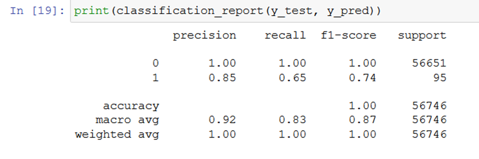
Since this data is imbalanced (having very less number of cases when y =1). In cases like this, the Classification report gives more information than simple accuracy measures. It tells about precision and recall as well.

          print(classification_report(y_test, y_pred))        

Step 5.4 – Visualizing using Confusion Matrix

Confusion Matrix also gives similar information to the classification report, but it is easier to understand. It shows how many values of each class were correctly or incorrectly classified.

          cm=confusion_matrix(y_test,y_pred) plt.figure(figsize=(12,6)) plt.title("Confusion Matrix") sns.heatmap(cm, annot=True,fmt='d', cmap='Blues') plt.ylabel("Actual Values") plt.xlabel("Predicted Values") plt.savefig('confusion_matrix.png')                  

Conclusion

There are different types of Logistic Regression, but the most widely used is the binary logistic regression in which the classification takes place on one of the two possible values of the target variable. Logistic Regression is different from Linear Regression because it is a classification algorithm and has discrete values as classification output, while Linear Regression is a Regression algorithm having continuous values as output. We also covered that Logistic Regression finds its use in a wide range of applications including the classification tasks in Business, Education, and Medical industries.

A real-life example of Logistic Regression was studied. The analysis involved over 280,000 instances of transactions which were further divided into training and test sets by a ratio of 80 to 20 respectively. After exploring and preprocessing the dataset, the model was trained and a classification accuracy of 99.9% was obtained. It showed that Logistic Regression was very successful in detecting fraudulent transactions, although more improvement can also be made by tuning the model (advance concepts).

If your project is based on AI or Machine Learning you should work with the best specialists. Meet our team and see how we can develop your software together.

knighthagerre.blogspot.com

Source: https://asperbrothers.com/blog/logistic-regression-in-python/

Share this post